Tutorial 5: Rinsing simulation
Description
Scope: In this tutorial, we will create a new workflow from scratch and assess how the adsorption of a surfactant on a cellulose surface is modified under the action of a rinsing cycle.
Difficulty: high
Time required: 15 minutes of setting the system + doing the NEXTMOL Builder tutorial Tutorial 3: Creating a surface is a prerequisite + 3 hours of computation.
Creating the chemical species
Given that the aim of the tutorial is to calculate the changes in the adsorption of a surfactant on a surface, let’s focus on the creation of these two species. The surface can be generated following the steps described in the tutorial Tutorial 3: Creating a surface. As for the surfactant, in this case a molecule of Sodium Dodecyl Sulfate or SDS is selected. Hence, the user must open the side menu, click on the 'Molecules' option and select 'New Molecule'. Note that at this point we will name the molecule 'Dodecyl Sulfate', as the sodium cation will be added separately in the workflow. Then, in the 'Designer' tab, the user can draw the following:
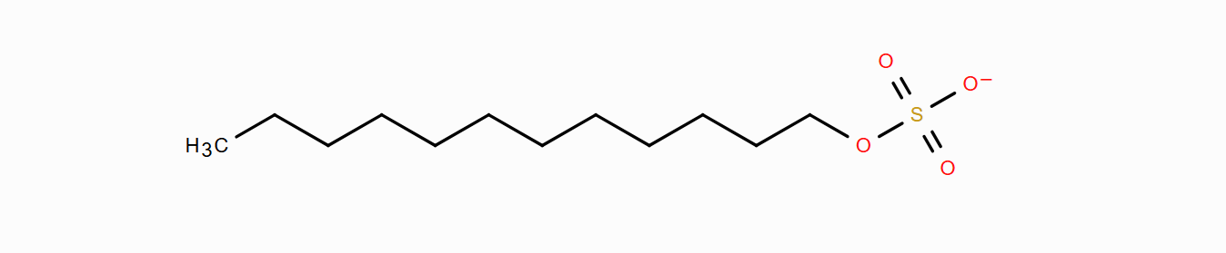 Figure 1. Dodecyl sulfate.
Afterwards, the molecule can be saved and generated. Lastly, the topology of dodecyl sulfate must be generated, for which a charge of -1 and the GAFF2 force field must be indicated at the 'Potentials' tab. By clicking on 'Run', the platform will generate the topology files of the molecules within seconds. Once these chemical systems have been generated, the construction of the workflow may be started, as the rest of the species that will appear in this tutorial as water or sodium cation appear by default in all the accounts.
Defining the workflow
The objective of this setup is to create a monolayer of surfactants in aqueous solution over a surface of cellulose. Therefore, next it is shown how to progressively build such a complex chemical system. The list of nodes in the workflow is described next for the sake of completeness, but building it from scratch is not absolutely necessary as the whole workflow is available in the list of provided pre-assembled workflows. Those parameters that are not directly mentioned in the following list may be left with its default value. Create a new project called 'Tutorial 5' and an experiment inside called 'Rinsing simulation'. If you wish to skip this section, click on 'Import workflow' and select 'Tutorial 5: Rinsing simulation' Otherwise, click on 'New workflow' and name the new workflow also "Rinsing simulation". Then, select the option 'Edit Workflow' and progressively add nodes to the workflow using the following list and clicking on 'Add step':
-
Node 1: 'Dodecyl sulfate' molecule.
-
Node 2: 'Orient system' system operation function, being the node 1 its parent. It can be called 'Orient downwards', as it orients the head of the surfactant downwards, where it will meet the cellulose surface. For that end, the 'O3' atom can be selected in the 'Atom name of reference atom' field.
-
Node 3: 'Translate' ystem operation function , being the node 2 its parent. The node may be called 'Move to origin', as it facilitates the placing of the molecule at the bottom of the simulation cell, which later on will facilitate the union of the surfactant monolayer with the cellulose surface. Thus, all the 'Origin point' and 'Target point' selectors can be set at 'min'.
-
Node 4: 'sodium ion' molecule.
-
Node 5: 'Insert system' system operation function, being the nodes 3 and 4 its parents. Note that two nodes can be selected at once while pressing 'Ctrl' in Windows or 'Control' or 'Command' in macOs. This node places the sodium ion next to the surfactant. Hence, this can be achieved by simply indicating '2' at the 'Target point x value'.
-
Node 6: 'Create layer' system operation function, taking node 5 as its parent. A monolayer of surfactants will be created out of this node. For that, indicate 70x70x50 Å3 in the cell dimensions and 'z' on the surface normal. Due to the operations coming from the previous nodes, the surfactants in the monolayer will be placed with their head pointing downwards. Finally, indicate 30 units in 'Total number of components for parent 1' and 1 for 'Minimum distance between the atoms of parent 1 and existing components'. It is important to note that the higher the coverage of the interface is, the lower the distance between inserted components must be, otherwise the specified amount of surfactants will not fit the simulation cell. In this case, 1 Å is low enough to easily accomodate 30 or more surfactants. Note that, while this intermolecular distance is too short, a later energy minimization will relax the initial geometry of the system.
-
Node 7: 'Modify cell size' system operation function , being node 6 its parent. This node will make space above the surfactant layer to accomodate the solvent molecules. For x and y dimensions, indicate 'manual value selection' for 'cell side' and 70 for each value. In the case of the z dimension, select 'set to system size (max-min)'. Activate the 'reposition system' option and set 'Target point z value' to 'min'. Finally, in the section 'Reference point for the repositioning', set all values to 'min'.
-
Node 8: 'Water TIP3P-FB' molecule.
-
Node 9: 'Fill cell' system operation function, taking nodes 7 and 8 as parents. This node will fill the simulation cell with water molecules. Thus, make sure that the 'Water TIP3P-FB' is second in the hierarchy list, indicate 6000 molecules for the total number of components of parent 2, set the minimum distance between inserted components to 1 Å and deactivate the periodic boundary conditions in z. This way we will consider periodicity only in the xy dimensions.
-
Node 10: 'Cellulose 70x70x30' molecule, created during Tutorial 3: Creating a surface.
-
Node 11: 'Join systems' system operation function, taking nodes 9 and 10 as parents. This node will join the monolayer of surfactants on top of the cellulose surface. Make sure that the cellulose surface appears first on the hierachy list, then indicate 'xy top' in the 'Sides to join' option and select 2 Å as buffer, i.e., an initial separation that will disappear during the simulations.
-
Node 12: 'Modify cell size' system operation function, taking node 11 as parent. This node aims to fix any potential previous mistake committed during the building of the workflow. Change the 'Cell size z' option to 'set to system size (max-min)'.
-
Node 13: 'Energy minimization' Gromacs simulation, which receives node 12 as a parent. This is the starting point of the simulations and it will avoid clashes between molecules. For this end, in the 'Run Parameters' section select 'Energy Minimization' and in the 'Thermostat' section deactivate the generation of random velocities.
-
Node 14: 'NPT equilibration' Gromacs simulation, using node 13 as a parent. During the execution of this simulation the geometry of the system will evolve from an artificial setup of randomly placed molecules to an experimentally equivalent setup at standard conditions. Check that the settings are indicated as follows:
-
Run parameters: set 'Calculation Mode' to 'Molecular Dynamics', the time step to 0.001 picoseconds and the number of steps to 1000000.
-
Output control: we recommend increasing the frecuency for writing to avoid excessively large output files during equilibration. Thus, indicate 50000, 10000 and 50000 in the trajectory, energy and 'log' frequency indicators.
-
Electrostatics: before opening the section, click on 'Show expert parameters' at the top of the node. Then, open the 'Electrostatics' panel and change the 'Geometry to perform the reciprocal sum' to '3d corrected'.
-
Thermostat: select the 'v_rescale' thermostat, a reference temperature of 300 K and a time constant for coupling of 1 ps. Also, activate the generation of initial velocities at 300 K.
-
Barostat: select the Berendsen barostat, indicate 'semiisotropic' at isotropy selector and reference pressures of 1 bar for both xy and z dimensions. As a general recommendation, it is a good idea to set the time constant for coupling of pressure five times bigger than that of the temperature, i.e., 5 picoseconds in this case.
-
PBC and neighbor search: change the peridic boundary conditions to 'surface periodic (xy)'.
-
Position restraints 1: in component 1 indicate the 'Dodecyl sulfate' molecule and apply restrictions of 500 kJ mol-1nm-2 to all dimensions. This will avoid the surfactant to desorb before the production run starts.
-
Potential Walls: set 'Number of walls' to 2 and use the default settings.
-
-
Node 15: 'NVT production' Gromacs simulation node. This is the simulation in which, having prepared a chemical system in experimentally realistic conditions, the adsorption of the surfactant on the surface will be assessed. To generate this node, instead of clicking on 'Add step', click on the 'NPT equilibration' Gromacs simulation node and then select 'Copy'. A copy of the previous node will be generated, on which the following changes must be applied:
-
Run parameters: increase the number of steps to 10000000.
-
Output control: reduce the writing frecuency of the trajectory, energy and 'log' to 10000, 1000 and 10000 respectively.
-
Barostat: deactivate the barostat by selecting 'No' in the 'Pressure coupling mode'.
-
Position restraints 1: in component 1 change the chemical species to the cellulose surface, which will be represented by a label starting by 'chain_1-'. This way the adsorption process will be easier to study.
-
-
Node 16: 'Adsorption on surface' post-processing node, using node 15 as parent. This will generate the analysis of the adsorption of dodecyl sulfate on the cellulose surface during the previous run. In the 'General' section, select the dodecyl sulfate molecule, indicate 'z' as the perpendicular direction to the surface and deactivate the option 'Use PBC in direction perpendicular to surface'. This node allows to select several surfaces or regions of the surface, but in this case only one is necessary. Go to 'Surface zone 1' and change the name of the zone to 'Cellulose'. Next, select the component name of the surface, which we kindly remember that is represented by a label starting by 'chain_1-'.
-
Node 17: 'NVT acceleration' Gromacs simulation node, which has also node 15 as a parent. This node will perform a new simulation in which an external force is applied on the water molecules, simulating a rinsing cycle. Copy node 15 and just change the following settings:
-
Acceleration: select the option 'Define using acceleration' in the 'Perform Acceleration' tab, change the name of the acceleration group to 'Solvent' and select the water molecules in the component name. Lastly, apply an acceleration of 1 pm/ps2 in the x axis.
-
-
Node 18: 'Adsorption on surface' post-processing node, using node 17 as parent. It may be directly copied from node 16.
Figure 2 presents a depiction of how the final workflow should look like.
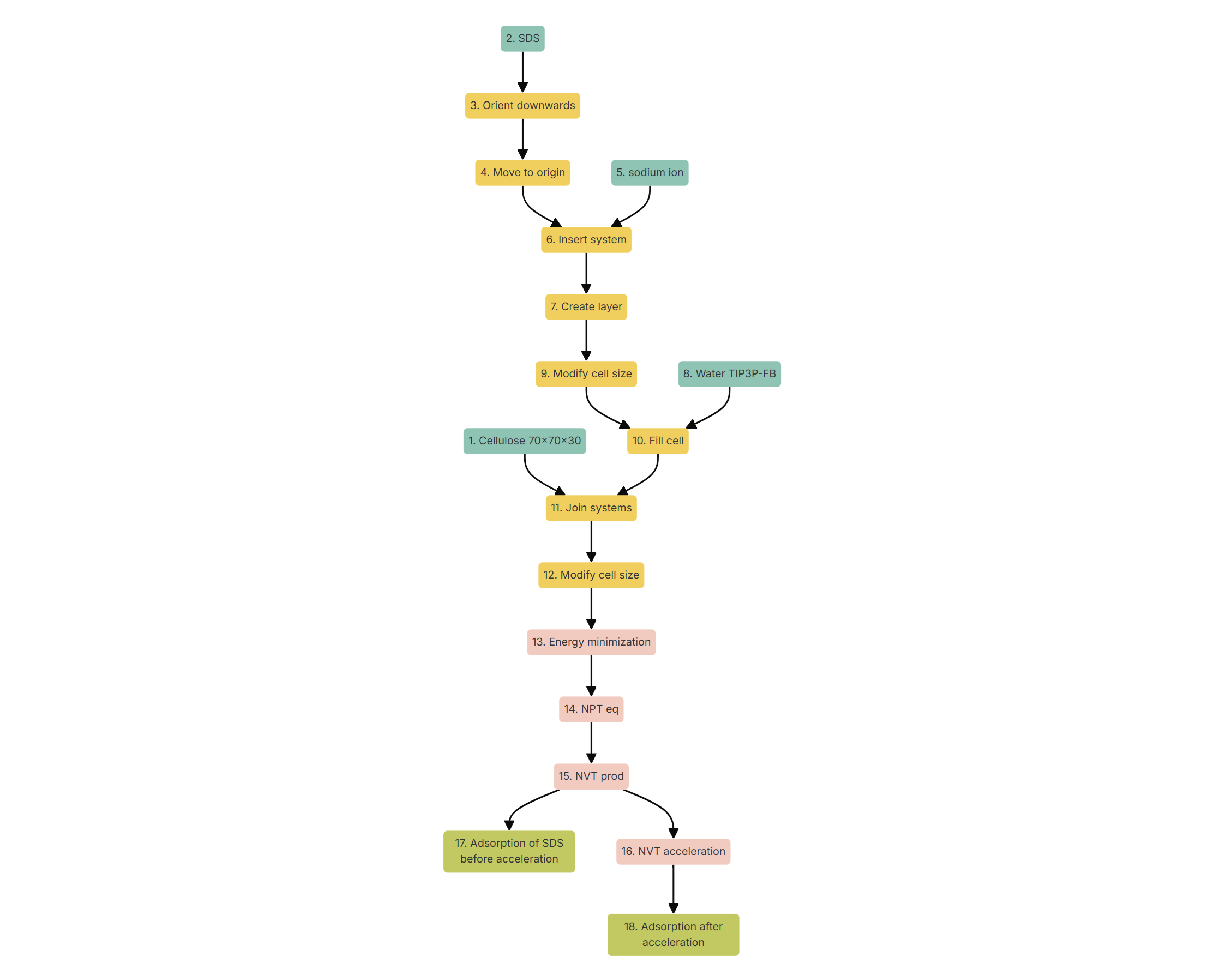 Figure 2. Computational protocol for the study of the effect of a rinsing cycle on the adsorption of a surfactant on a surface.
Running the simulation
Once the workflow is ready, click on nodes 16 and 18, i.e., both post-processing nodes, while holding 'Ctrl' (or 'Command' if you are using macOS) to effectively select both nodes. Then, click on 'Create job', name the new job and save it. Finally, execute the simulation, which should take about 5 hours without considering queue times that may vary depending on the availability of the computational resources. Next, a snapshot of the chemical system before (left) and after (right) the simulations is shown:
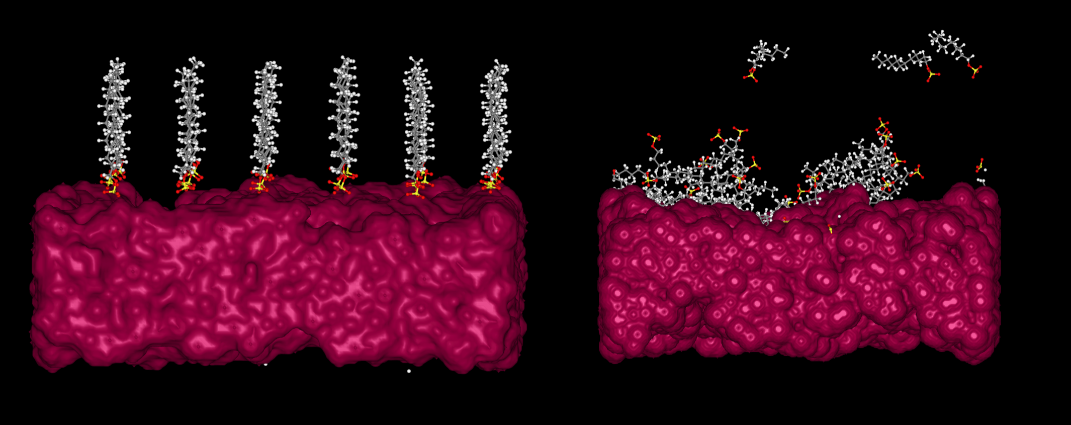 Figure 3. Representation of a monolayer of dodecyl sulfate molecules on a cellulose surface before (left) and after (right) the simulations defined in Figure 2.
Analyzing the adsorbance
Once the job is done, enter the job and click on node 16. Then, click on the blue 'New analysis' button at the top and select the 2D option. A new window will appear, allowing the user to define a new two-dimensional analysis regarding the adsorption of dodecyl sulfate on cellulose before the rinsing cycle. Select 'Time' in the x axis and '% of adsorbed residues of the molecules'. Finally, name the analysis as 'Adsorption before rinsing' and save it. After few seconds, the analysis will be ready to visualize:

Figure 4. Time evolution of the percentage of adsorbed residues of dodecyl sulfate during the 'NVT production' Gromacs simulation node.
The equivalent protocol can be followed for the analysis of the adsorption of dodecyl sulfate on cellulose after the rinsing cycle:

Figure 5. Time evolution of the percentage of adsorbed residues of dodecyl sulfate during the 'NVT acceleration' Gromacs simulation node.
Thus, it can be observed how the rinsing cycle eliminates part of the dodecyl sulfate that was steadily adsorbed on top of the cellulose surface. Please, note that for the sake of simplicity and quickness, the simulated system has been limited in size. This can serve as the foundation to create more sophisticated experiments: comparison between the adsorption strength of different surfactants, performance of surfactant blends, influence of changing the surface or the temperature and more. If you are interested in these properties or you would like to create a more complex version of this workflow, please do not hesitate to contact us at support@nextmol.com .