Radius of Gyration
The Radius of Gyration (Rg) in Molecular Dynamics simulations is a measure of the size and compactness of a structure across the duration of the simulation. Usually applied to polymers or peptides, the Rg is defined as:
where N is the number of atoms or particles and ri2 is the position of the i-th atom relative to the center of mass of the molecule.
Scientific implementation
The radius of gyration is computed through the calculation of the gyration tensor. The gyration tensor is a symmetric 3x3 matrix in which each element is computed following the formula:
where N is the number of atoms or particles, rm(i) is the m-th cartesian coordinate of the position vector of the i-th particle, and rn(i) is the n-th cartesian coordinate of the position vector of the i-th particle. The origin of the coordinate system is the center of mass of the molecule, which means that to each component of the atom position vector, one has to subtract the corresponding component of the center of mass.
In terms of code, we iterate over the particles and add the corresponding multiplication of the position vectors to Smn and finally divide by the number of atoms to obtain the gyration tensor. The gyration tensor is then diagonalized. The sum of the eigenvalues returns the squared radius of gyration.
From a practical point of view, at each frame across a simulation trajectory, the atom group of interest (i.e., the polymer) is selected and the radius of gyration is computed individually and averaged over the number of molecules in the group. This approach ensures that the implementation works for both a polymer in solution and a polymer melt containing multiple polymer chains.
Computing Rg for a polymer in solution
A workflow is provided in the platform to compute the radius of gyration of a single polymer in solution. This workflow consists of 8 steps: the initial step, one system operation step, five simulation steps, and a post-processing step:
-
Initial step → Molecule selection: in this step, the molecules that form the system are selected. One will be the polymer, previously generated using the polymer builder tool. The other will be the solvent. To use a mixture of solvents, one will need to add extra molecules and slightly modify the next step.
-
System Operation → Build Solvated Polymer: it has two parent steps that are the molecules that form the system, namely the polymer and the solvent (in the case of a mixture of solvents, the number of parents would be increased). Based on the weight of the polymer, one may need to change the concentration of the components to get a system with a single polymer chain. Concentrations between 1.5% and 3.0% should work, but it depends on the molecular weight of the polymer. At this point, the user is encouraged to increase the cell size (defaults to 5x5x5 nm3) if using a big polymer chain, and to adapt the density field to match that of the solvent at hand.
-
Simulation Operation → Minimization: performs an energy minimization to relax the initial configuration and avoid any possible initial clashes between the molecules.
-
Simulation Operation → NVT equilibration: performs an equilibration in the NVT ensemble, that is keeping the number of particles, the volume and the temperature constant. This step will bring the system to the desired temperature (default = 300K), allowing the solvent to reorganize around the solute.
-
Simulation Operation → NPT equilibration 1: performs an equilibration in the NPT ensemble, that is keeping the number of molecules, the temperature and the pressure constant. A pressure of 5 bar is used in this step to compress the system and eliminate any possible voids or gaps in the box.
-
Simulation Operation → NPT equilibration 2: performs a second equilibration in the NPT ensemble at 1 bar. This step will bring the system to the desired density.
-
Simulation Operation → NPT Production: a final NPT simulation step of 10 ns long that will be used to compute the radius of gyration.
-
Post-processing → Rg Calculation: in this step, the radius of gyration is calculated. It is important here that the component name matches the name given to the polymer.
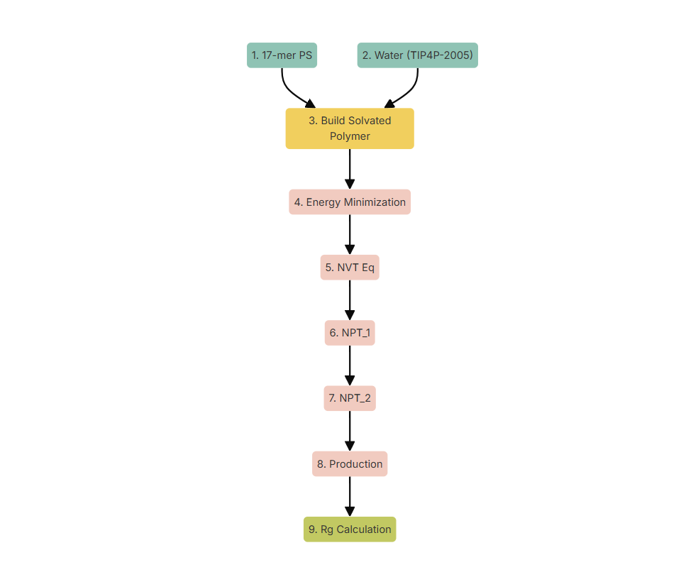 Figure 1. Workflow for the calculation of the radius of gyration of a polymer in solution.
Computing Rg for a polymer melt
A workflow is provided in the platform to compute the radius of gyration of a polymer melt formed by several chains of polymer. Since Rg heavily depends on the molecular weight of the polymer, it is suggested to use a melt formed by polymer chains of the same length. The workflow has an initial step, followed by 7 simulation steps and a post-processing operation:
-
Initial step → Molecule selection: in this first step the system to be simulated is selected, which in this case corresponds to a polymer melt generated with NEXTMOL Builder.
-
Simulation Operation → Energy Minimization: performs an energy minimization to relax the initial configuration and avoid clashes or overlaps between the polymers.
-
Simulation Operation → NPT equilibration 1: equilibration step at 100 bar to remove any possible voids created by the random walk process of the polymer builder.
-
Simulation Operation → NPT equilibration 2: equilibration step at 1 bar to get to the desired density.
-
Simulation Operation → NPT Heating: the system is heated from 300 K to 1000 K via a 100 K/ns ramp and then the temperature is maintained at 1000 K for one more nanosecond.
-
Simulation Operation → NPT Cooling: the system is cooled from 1000 K to the desired final temperature (default 300 K) using a cooling ramp of 18.42 K/ns. The system is then kept at the desired temperature for 2 ns.
-
Simulation Operation → NPT equilibration 3: final equilibration process at the desired temperature and 1 bar for 10 ns.
-
Simulation Operation → NPT production: final NPT run at desired temperature and 1 bar for 10 ns.
-
Post-processing → Rg calculation: computes the Rg for the specified component. In this case, the calculation may take longer since the Rg is computed for each chain and averaged.
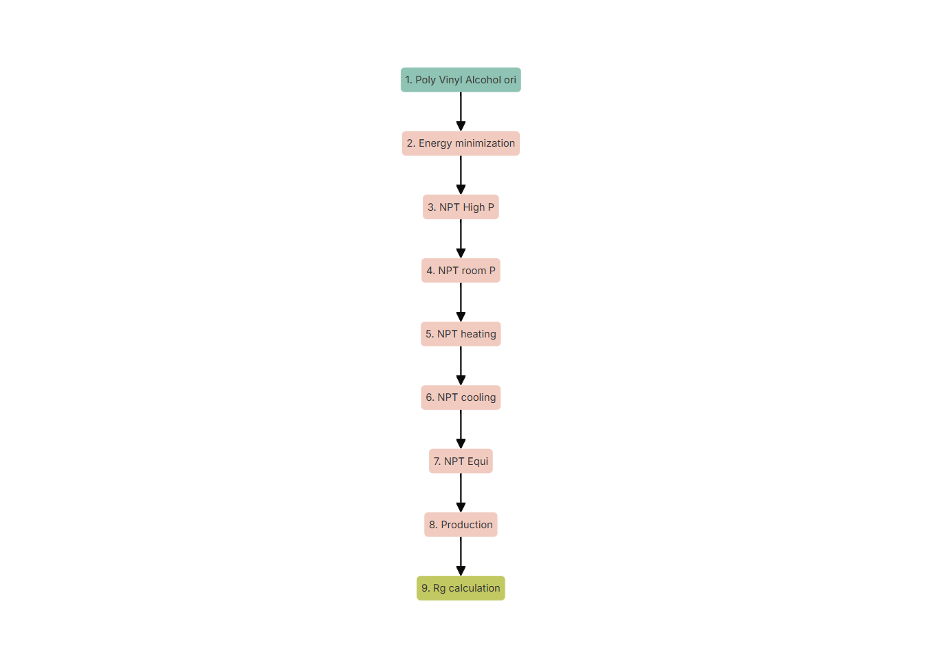 Figure 2. Workflow for the calculation of the radius of gyration of a polymer melt.
Analysis of the results
After running the workflow, to visualize the results one needs to select the Rg calculation node, go to NEW ANALYSIS and select 2D in the dropdown menu. Then choose time for the X axis and radius of gyration for the Y axis. The analysis provides the time evolution of the radius of gyration along the production simulation. Below you can find an example for a polymer in solution and for a polymer melt (Figures 3 and 4 respectively).

Figure 3. Time evolution of the radius of gyration of a polymer in solution.

Figure 4. Time evolution of the radius of gyration of a polymer melt.