Tutorial 4: Glass Transition Temperature of Polyethylene

Scope: In this tutorial, we will create a new workflow from scratch and calculate the glass transition temperature of polyethylene.

Difficulty: medium

Time required: 10 minutes of setting the system + doing the NEXTMOL Builder tutorial Creating a linear polymer is a prerequisite + 3 hours of computation.

Firstly, we can create a new project called 'Glass Transition Temperature' and a new experiment called 'Polyethylene'. The workflow will be started from scratch, so we can create a new workflow and name it '10 chains of polyethylene'. We are using this system as this is the product of the NEXTMOL Builder Tutorial Creating a linear polymer. In order to use it in a workflow, we must first import it. Click the button on the top-left corner of the screen and click on 'Molecules'. In the top-right corner of the molecules section you can click on 'Import Molecules' and you will see the complete list of molecules and systems that have been processed in your NEXTMOL Builder account. Search for '10 chains of polyethylene' and click on import, incorporating this system into your list of available molecules in NEXTMOL Modeling.

Go back to the '10 chains of polyethylene' experiment, click on 'Edit workflow' and then on 'Add molecule'. Search the '10 chains of polyethylene' system and click on 'add'. You can visuzalize the chains of polyethylene (Figure 1) by clicking on its node and then clicking on 'Edit Step'.

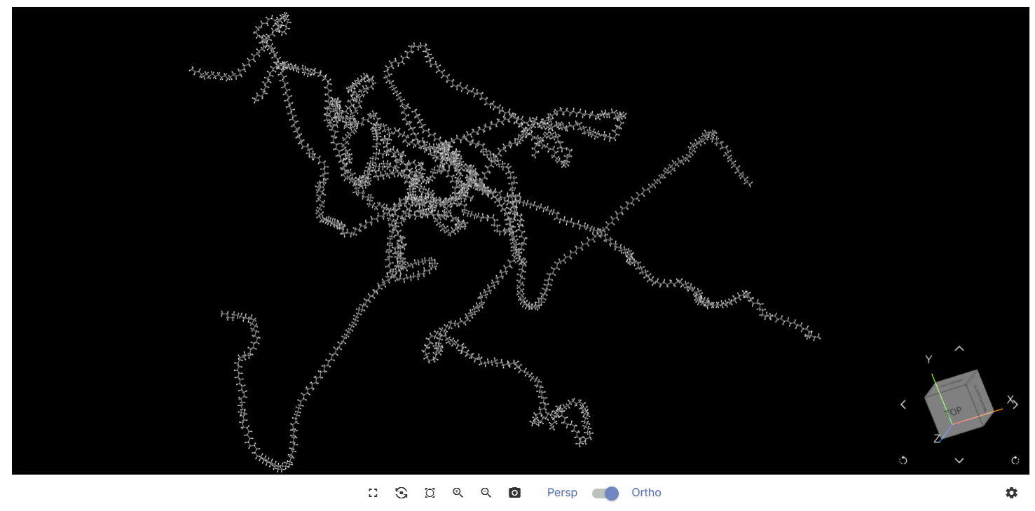Figure 1. Chains of polyethylene.

Next, we are going to define the sequence of nodes of simulation of our workflow. It is composed by: an energy minimization, which will correct any excessively large force in the inital geometry; two NPT equilibrations, which will first compress the system with a pressure of 20 bars and then equilibrate it at 1 bar; a quick NPT heating until 1000K; another quick NPT node to equilibrate the system and finally an NPT production node in which the system will cool off from 1000K to 50K. The settings for each node are as follows (select default values for the parameters that do not appear in the list):

Finally, we can add a 'Glass Transition Temperature' post-processing node.

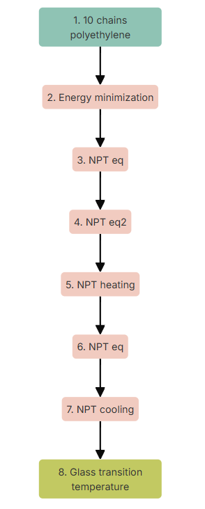
Figure 4. Workflow of the experiment.

We select the post-processing node and click on 'Create job'. We run the calculation with default settings. The simulation nodes will take at least three hours, depending on the availability of the computational resources. Once the job is completed, we can go to the job page, click on the 'Graph' tab, select the 'Glass Transition Temperature' and click on 'View step'. There you will be able to download the 'props_values.json', which contains the glass transition temperature of polyethylene according to two different approaches, a fitting of the density vs temperature data to a hyperbolic function and as the intersection of two tangents adjusted to two different regimes. In both cases, we obtained a glass transition temperature of 359K, indicating that the calculations are converged.