Tutorial 3: Interfacial tension water/surfactant/oil

Description

Scope: In this tutorial we will calculate the interfacial tension of an oil/water system with surfactants at the interface between the two phases. Starting from a pre-configured workflow, we will show how to change the type of surfactant, the number of surfactants in the preassembled layer at the interface, and how to run and visualize the simulations. In order to learn how to create a project and workflow from scratch, we refer to tutorials 01 and 02.

Difficulty: easy

Time required: 30 minutes (up to 1 day of simulation time)

Pre-requisite: Tutorial 01 and Tutorial 02

Introduction

Due to their amphiphilic nature, surfactants adsorb at the boundary between two immiscible phases and reduce the Interfacial tension (IFT) between them. The reduction of the IFT between the phases depends on the surfactants concentration, which in turn alters the number of adsorbed surfactants per area at the interface.

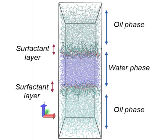
In our model, the IFT of a water/surfactant/oil system is computed using a preassembled model of oil and water phases with a monolayer of surfactants in between them, with the interface normal oriented along the z axis (see scheme in Figure 1). Then, after a Molecular Dynamics (MD) run in the NPT ensemble, the IFT is calculated from the diagonal components of the pressure tensor as the difference between the component orthogonal to the interface (z-component in the simulation, Pzz) and the components parallel to it (x- and y-components, Pxx and Pyy): γ=Lz/2(Pzz−1/2(Pxx+Pyy)), with Lz being the length of the simulation cell along the z-direction.

Figure 1. Simulation model.

Preparing the working environment

The first task is to set up the project where the work will be executed. Go to the icon-hamburger placed at the top left corner of the screen, and select Projects. Here you will find the list of projects under your profile. You can either create a new project with the NEW PROJECT button or choose one of the existing ones. For this tutorial, let’s create a new one.

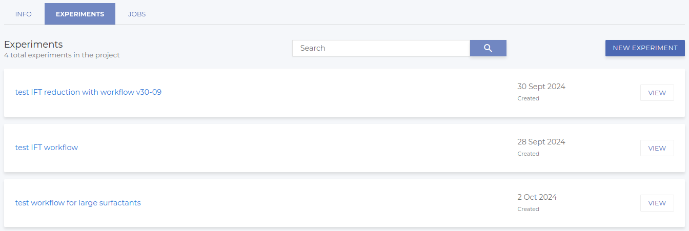
Inside the project folder, you will find the EXPERIMENTS tab where you can manage and create your experiments (see an example in Figure 2). Since we have created the project from scratch, there are no experiments yet, so we have to create a new one via the button NEW EXPERIMENT.

Figure 2. Experiments page.

After filling in some basic information, you will be asked whether you want to start the experiment from scratch (NEW WORKFLOW) or import an existing workflow (IMPORT WORKFLOW). Here we choose the second option to import the workflow that has been prepared for this tutorial; out of the available workflows choose the one called “Interfacial Tension v2024-10-03”

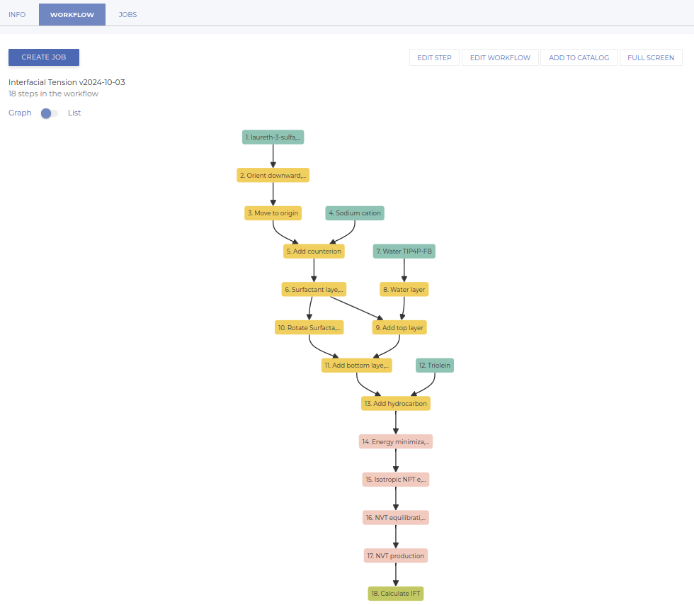
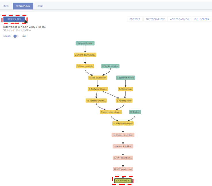
Once the workflow has been imported, you access three tabs: INFO (where you can change the name and description of the experiment if desired), WORKFLOW and JOB. In the WORKFLOW tab you will see the preconfigured workflow containing all the steps needed for the calculation of the interfacial tension. It should look like the one represented in Figure 3.

Figure 3. The imported workflow.

Modify the existing workflow

Now let’s edit the workflow by clicking the EDIT WORKFLOW button. Here two new tabs become available: INFO, where you can modify the name, the tags and the description of the workflow, and GRAPH, where you can visualize all the nodes of the workflow and modify them as desired. Let’s go to that one.

The workflow has been prepared and tested in order to be stable and yield accurate results. Yet, any node of it can be edited if desired (even nodes can be added or deleted, but this goes beyond the scope of this tutorial). However, in a typical use case, only the following variables will be modified from one experiment to another:

the type of surfactant that is used;
the number of surfactants that are arranged at the surface;

Change the type of surfactant

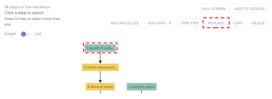
First, let’s change the surfactant molecule. To do so, select the first node (click on it) and then click on REPLACE, as shown in Figure 4.

Figure 4. Change of surfactant.

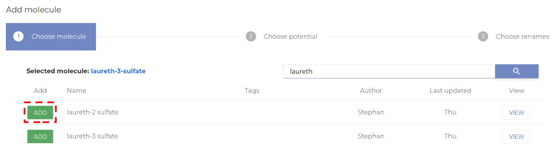
This opens a three-step wizard to select the new molecule. In the first step, you can choose the molecule from the catalog of available molecules. Once you have identified that molecule you want, click on ADD, as shown in Figure 5. In the subsequent steps of the wizard, you can choose the potential that you want to use for the simulation (in many cases there is only one), and in the last step you can optionally rename the molecule.

Figure 5. Molecule selection.

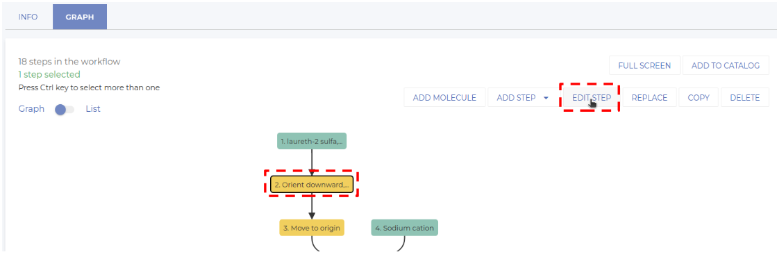
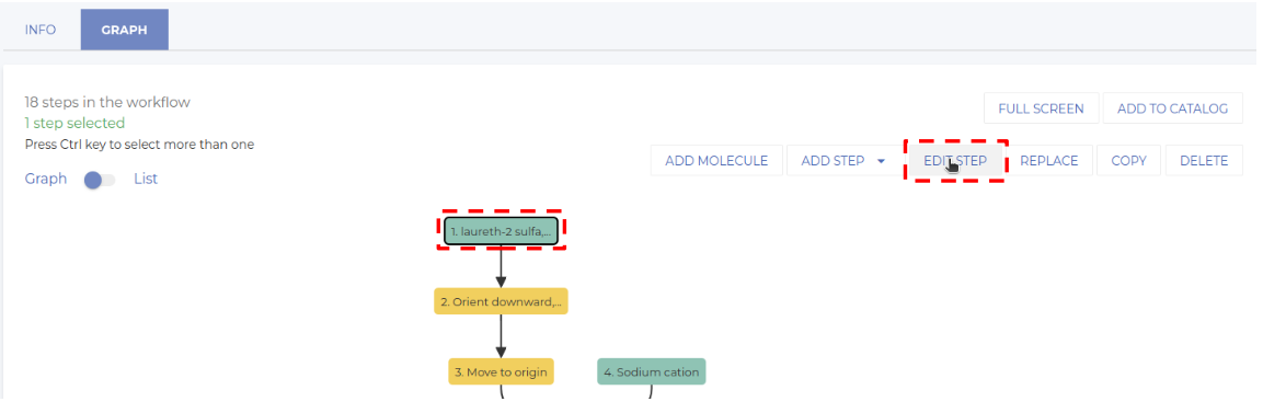
There is an important detail that one has to pay attention to when switching the molecule. Right after the initial node with the surfactant, there is a node that orients the molecule so its polar head points downwards. This node has to be adjusted when a new molecule is used. To do so, select the node and click on EDIT STEP, as shown in Figure 6.

Figure 6. Select second node.

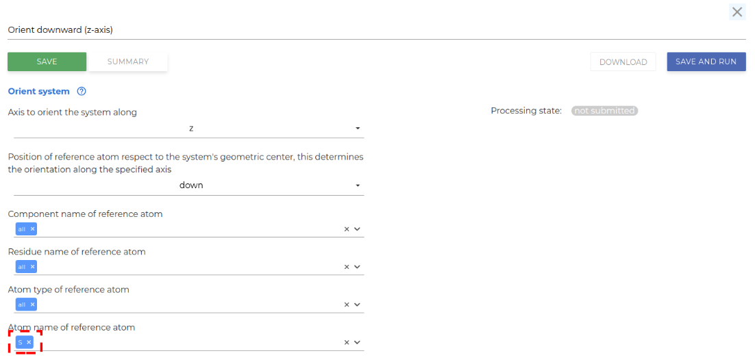
The function to be edited selects a (group of) atoms and orients the surfactant such that this group points downwards along the z-axis. Hence, every time a new molecule is studied, one has to redefine that reference group of atoms. This can be achieved via the multi-selector shown in Figure 7. In our specific case, it is enough to select any atom of the polar head group (here for instance S; see the next paragraph to learn how to obtain this information). Once done, click on SAVE and exit by clicking on the cross in the upper right corner.

Figure 7. Select atom.

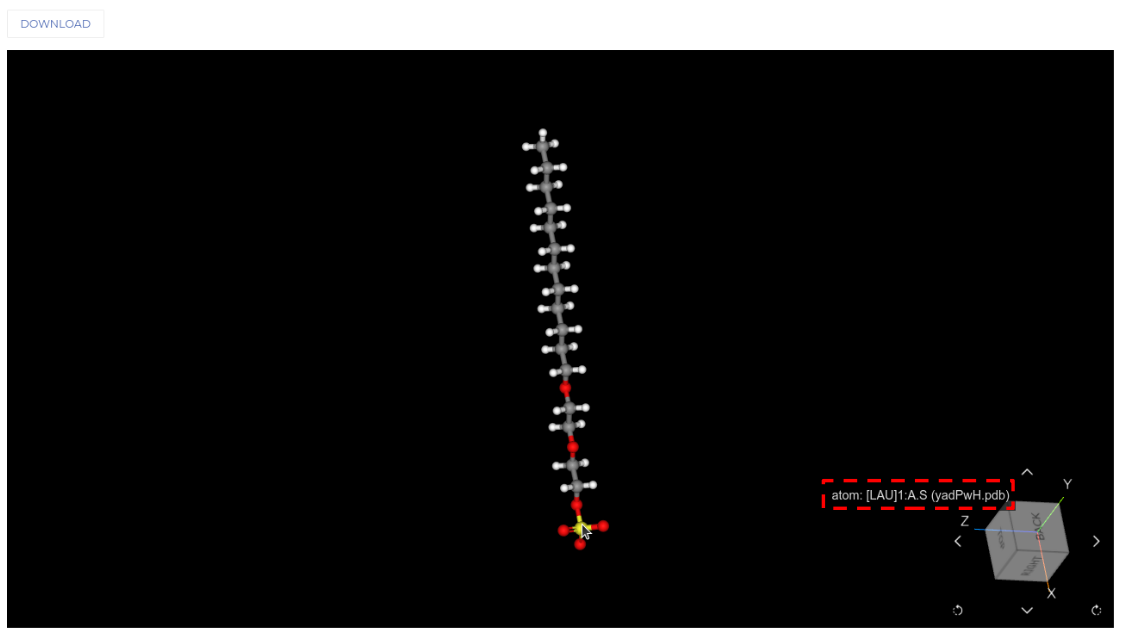
In order to know which atom should be selected, select the surfactant molecule node and click on EDIT STEP, as visualized in Figure 8.

Figure 8. Check molecule.

This opens a 3D visualization of the molecule. Hovering the mouse pointer over the atoms displays their name, as indicated in Figure 9. The last name (after A.) indicates the name that can be used to orient the molecule.

Figure 9. Check atom.

Change the number of surfactants at the interface

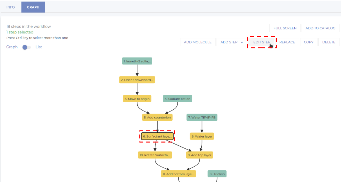
Next, we want to adjust the number of surfactants in the monolayer. To this end, we select the node “surfactant layer” and click on EDIT STEP, as visualized in Figure 10.

Figure 10. Change surfactant layer.

Figure 11. Change surfactant layer.

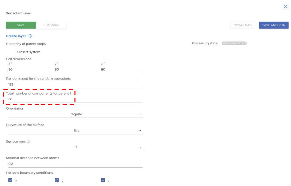
This displays all options of this node. As indicated, we want to change the number of surfactants; to do so you have to modify the value of “Total number of components for parent 1” (see Figure 11), and then save your changes by clicking on SAVE. Please note that very large values (exceeding the number of molecules that fit in a monolayer) will lead to failures. Apart from only saving the parameters, it is also possible previsualize the layer; to do so, click the SAVE AND RUN button, which will interactively execute the workflow up to the current node and then display the resulting system on the right hand side of the current window. Depending on the size of the system and the current load of the computational resources, this process may take up to a few minutes. Once everything is set correctly, we can go back to the workflow by clicking on the cross in the upper right corner.

Execute the simulation

Now that the workflow has been set up, we can execute it. First, close the workflow by clicking the CLOSE WORKFLOW button. Then select the last node of the workflow and click CREATE JOB to launch the calculation, as shown in Figure 12.

Figure 12. Create job.

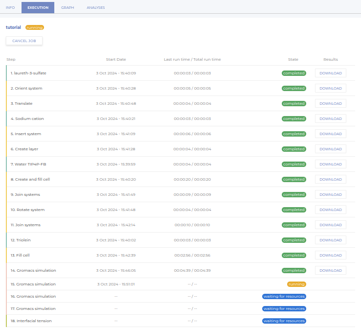
This opens a dialog where you can indicate a name and description of the simulation you want to execute. It is also possible to select the computational setup and reuse previous results, but for the time being these fields can remain at their default value. Once everything is set, click on the SAVE button, which activates additional tabs. Go to the EXECUTION tab and click on the EXECUTE JOB button. Once the simulation is launched, it will automatically execute all nodes of the workflow; the progress can be tracked in the EXECUTION tab, as shown in the example in Figure 13. It is possible to leave the current experiment and even the platform while the simulation is running. Once the simulation has finished, the platform will send you an email and you can go and check the outcome.

Figure 13. Job progress.

Analzyze the simulation

Obtain the IFT value

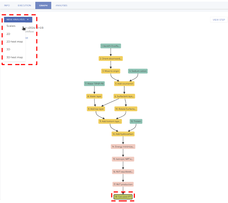
Once the simulation has terminated, we can check the calculated value of the IFT. To do so, go to the GRAPH tab, select the final node, and click on NEW ANALYSIS > Scalars, as visualized in Figure 14.

Figure 14. New analysis.

This opens a dialog where you can indicate a name and description of the specific analysis (e.g. “IFT”); then click on SAVE. After a few second, the RESULTS tab becomes active; switch to it to see the calculated IFT value. Please note that apart from the IFT, also some other quantities are displayed.

Carry out additional analyses

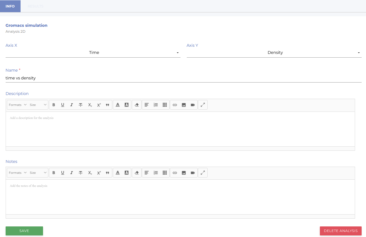
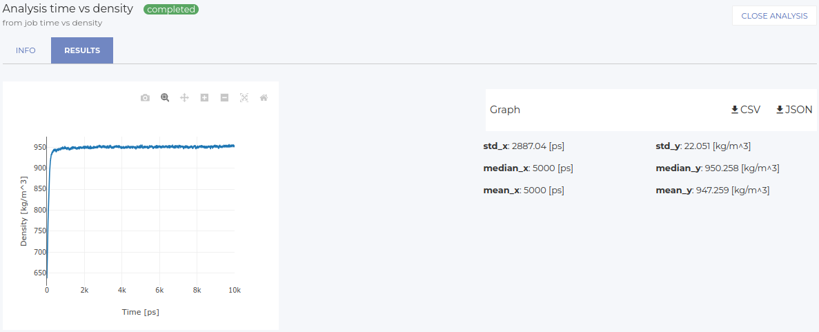
In addition, it is also possible to analyze additional properties on-the-fly. To do so, select one of the simulation nodes (the ones with reddish color) and click on NEW ANALYSIS > 2D. This opens a dialog where you can indicate the quantities to be analyzed via a 2D plot, e.g. time vs density (see Figure 15). Click on SAVE to launch the analysis; after some seconds the results are available in the RESULTS tab (an illustrative example is shown in Figure 16). The plot can be analyzed interactively, and it is also possible to download the results using the icons at the right.

Figure 15. 2D plot selection.

Figure 16. 2D plot.

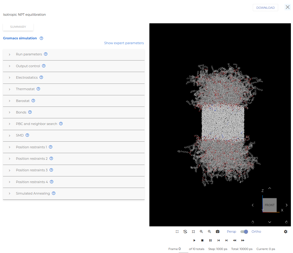
Visualizing the trajectory

Finally, it is also possible to visualize the trajectory of the MD simulation. Once the simulation has finished, go to the GRAPH tab inside the job, select one of the simulation nodes (the ones with reddish color), and select VIEW STEP. This will open a view that shows on the left the parameters of the node, and on the right a visualization of the system (see Figure 17). The buttons below the visualization window allow to visualize the entire trajectory. Please note that depending on the size of the simulation and your internet connection, this process can take some time.

Figure 17. Trajectory.