Tutorial 2: Adsorption at Clathrate-Hydrocarbon Interface
Description
Scope: In this tutorial we will study the adsorption of a small molecule (dodecyldimethylamine) at the interface between a clathrate surface and a liquid phase consisting of a hydrocarbon mixture. The molecule will initially be solvated in the dodecane phase, and we will gradually pull it toward the clathrate surface while calculating the Potential of Mean Force (PMF) using Steered Molecular Dynamics (SMD).
Difficulty: medium
Time required: 40 minutes (and up to two hours of simulation time)
Pre-requisite: Tutorial 01
Creation of the simulation system
Before performing any calculations, we need to create the system to be simulated. The system consists of a clathrate surface in contact with a liquid hydrocarbon phase containing the dodecyldimethylamine molecule, the adsorption of which will be studied. All components of this system are already available in the molecule catalog and can be imported via the ADD MOLECULE button:
-
Clathrate (TIP4P-ice/TraPPE-UA)
-
Dodecyldimethylamine
-
Dodecane-TraPPE-UA
-
Propane-TraPPE-UA
-
Ethane TraPPE-UA
-
Methane TraPPE-UA
You need to add these molecules, six in total. Please note that we are using a united atom model for the hydrocarbon phase to speed up calculations.
Now we can start building our system. There is not a single unique way to do it, but one possible solution is the following one:
-
Create a 2×2×1 supercell of the Clathrate crystal: This will be our surface. Use the Build supercell function and set the replication factors to (1,1,0).
-
Create empty space above the surface: This is where the molecule and the hydrocarbon molecules will be placed. Use the Modify cell size function to enlarge the box by 5 nm (50 angstrom) in the Z dimension, using the increase_value mode. No repositioning is required.
-
Insert the Dodecyldimethylamine Molecule: Now we insert the molecule at the desired position, i.e. centered in the X and Y dimensions, and at value of 3.5 nm in the Z dimension. Since the surface has a thickness of about 1.7 nm, this means that it will be located at about 1.8 nm above the surface. This can be achieved with the Insert system function, taking as reference point for the insertion the atom with atom name N and placing it at the center of the cell in the X and Y dimension and at value 3.5 nm in the Z dimension. A summary of the input parameters is:
-
Hierarchy of parent steps: 1. Modify cell size 2. Dodecyldimethylamine
-
Reference point of the inserted system: (geocen, geocen, geocen) for an atom with Component name "INH", Reside name "INH", Atom type "n3", and Atom name "N".
-
Insertion point: (center, center, value=35)
-
-
Embed the Molecule in the Hydrocarbon Phase: Use the Fill cell function to successively insert 100 dodecane molecules, 80 methane molecules, 12 ethane molecules, and 8 propane molecules. Insert each molecule with random position and orientation, ensuring a minimum distance of 2 angstrom between atoms, with PBC
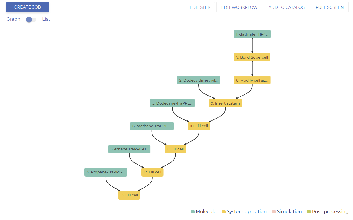
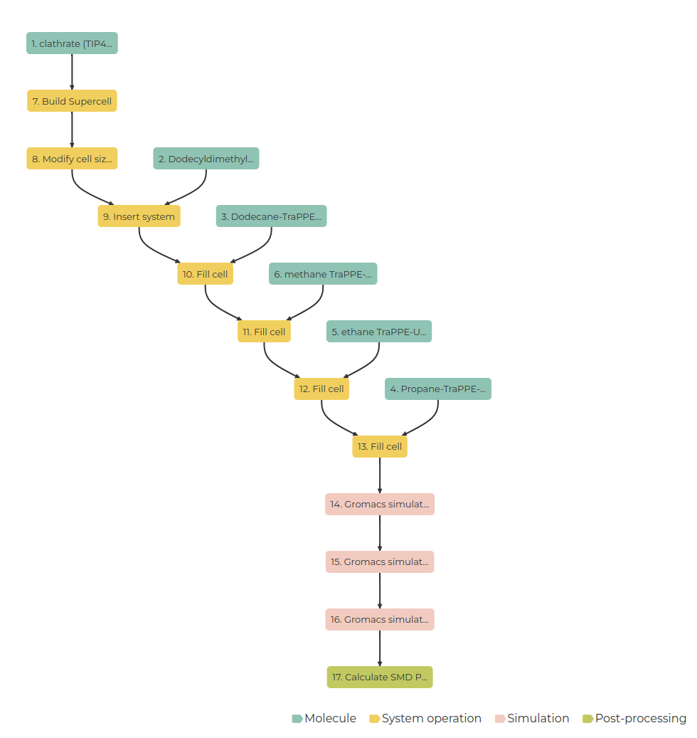
Your workflow should resemble the image below.
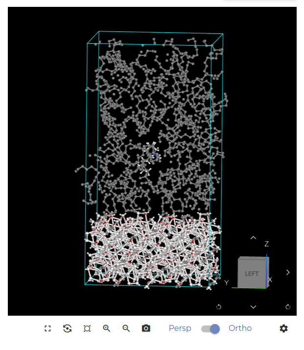
Let’s check that the system is correctly created. Select the last node (Fill cell), click EDIT STEP to enter that node and click SAVE AND RUN. This starts the creation of the system, and after about five minutes, you should see a visualization similar to the image below.
Set up of the simulation steps
Now that the system has been created, we will proceed with an energy minimization step to relax any unfavorably placed atoms, followed by a short MD simulation to adjust the box size according to the desired pressure.
-
Energy Minimization: Add a Gromacs simulation node and, under Run parameters > Calculation mode, select Energy minimization to perform an energy minimization using the steepest descent algorithm. Leave other parameters at default.
-
MD Simulation in the NPT Ensemble: Add another Gromacs simulation node, and modify the following parameters, leaving the rest with their default values:
-
Run parameters:
-
Calculation mode: Choose Molecular Dynamics instead of Energy Minimization.
-
Number of steps: 1,000,000
-
Time step: 2 fs (resulting in a simulation time of 2000 ps)
-
-
Output control: These values determine how often the code writes to the output files. The following numbers give reasonable results:
-
Frequency for trajectory writing: 50,000
-
Frequency for energy writing: 500
-
Frequency for log writing: 500
-
-
Electrostatics: Since the platform uses GPUs instances, please set VdW calculation mode to Cut-off.
-
Thermostat: Use the v_rescale thermostat at 277 K, with an initial velocity generation at 277 K. Set the coupling time constant to 0.1 ps.
-
Barostat: Use the semi-isotropic C-rescale coupling at a pressure of 100 bar. Important: activate the Expert parameters and set the compressibility in X/Y to 0. Use a 0.5 ps time constant for the coupling.
-
Position Restraints 1: Apply a position restraint to the OW1 atoms of the WATH component using a 1,000 kJ/mol/nm2 force constant. This will be enough to keep the structure of the clathrate slab fixed.
-
Position Restraints 2: Apart from the clathrate surface, we also want to keep the position of the molecule fixed (if we allowed it to move around freely it might adsorb before starting the SMD simulation). Apply a position restraint to the N atom of the INH molecule in the Z direction with a 500 kJ/mol/nm2 force constant to prevent premature adsorption.
-
-
SMD Simulation in the NVT ensemble: Now that the size of the simulation box has been adjusted to the applied pressure, we can launch the SMD simulation. Again, we will use a Gromacs simulation node, however this time in the NVT ensemble (i.e. no pressure coupling) in order to keep the size of the simulation cell fixed. The parameters are the same as those for the previous node, with the following exceptions:
-
Run parameters: We now use 10,000,000 steps with a time step of 0.002 ps. This yields a simulation time of 20 ns.
-
Thermostat: No initial random velocities are generated.
-
Barostat: No pressure coupling is applied.
-
Position restraints 2: no restraints are applied on the molecule.
-
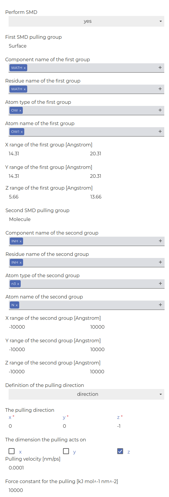
SMD:
-
Define two pull groups:
-
First group: The surface defined as the center of mass of some OW1 atoms of the water molecules in the center of the clathrate crystal (for instance, use the following ranges: X: [14.31:20.31]; Y: [14.31:20.31]; Z: [5.66:13.66])
-
Second group: The molecule defined via the N atom.
-
-
Set the pulling direction to negative z , define the velocity, and set the force constant (refer to image below).
-
-
The post-processing step and the workflow execution
The final step is to post-process the SMD data. This can be done with the Calculate SMD PMF node. Set the filter length and stride to 1,000 and 1, respectively, the lower integration bound to 50, and the spacing for the PMF function to 0.1.
If all steps are done correctly, your workflow graph should resemble the image below.
To execute the workflow:
-
Click on the last node and click CREATE JOB.
-
In the Execution tab, click EXECUTE JOB. The job should take 1–2 hours, depending on the available computational resources.
Analyzing the Results
To check the results, select the final node and click on New Analysis > 2D.
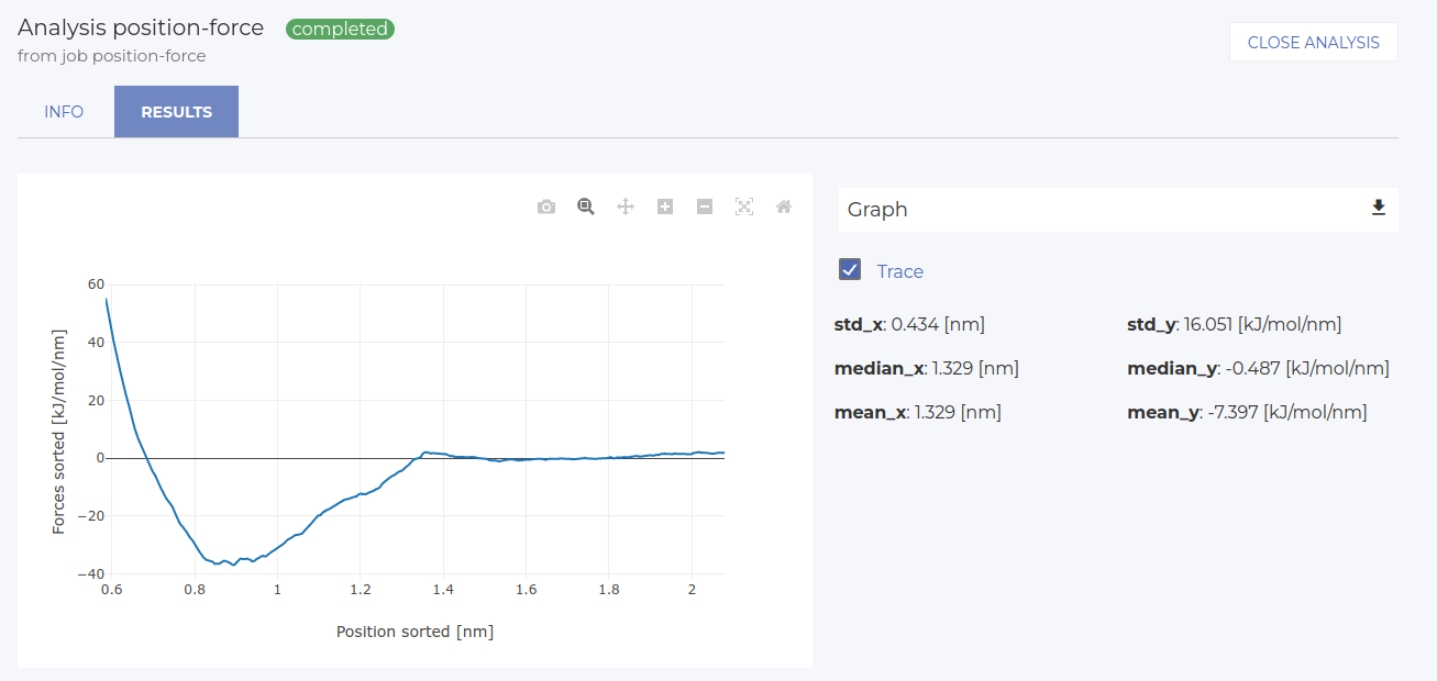
First, let’s visualize the position-force profile (select position_sorted vs forces_sorted). The result is in the image below. The x-axis shows the position respect to the center of mass of the first pulling group (selected in the last simulation step). Our particular choice leads to the center of mass in the z direction at about 0.85 nm. Therefore, the zero of the x-axis in is at z=0.85 nm of the simulation cell. Starting from the furthest distance, we see a clear adsorption well (attractive region, negative forces), followed by a steep repulsive region where the molecule is pulled into the surface (x=0.85 is the position of the interface).
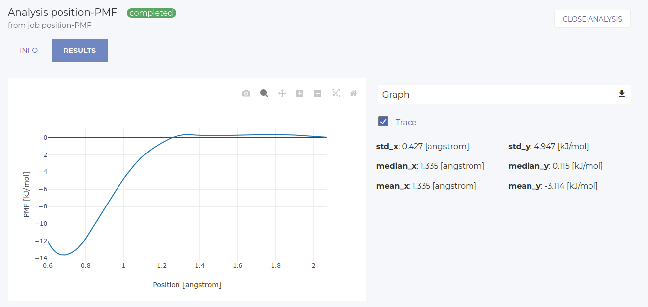
Subsequently, we can also look at the PMF profile. Select the final node again and click on New Analysis > 2D. Let’s visualize position vs PMF. The PMF is simply the integral of the position-force profile. Results are in the image below. The x-axis is the same as in the previous analysis. The minimum of the PMF profile corresponds to the adsorption free energy, i.e. DeltaG.