Tutorial 1: Density of Heptane
Description
Scope: In this tutorial, we will calculate the density of heptane by inserting a set number of heptane molecules into a box and running an NPT simulation.
Difficulty: easy
Time required: 10 minutes
Preparing the working environment
The first task is to create a new project. To do this:
-
Click the
 button on the top-left corner of the screen and click on Projects. You are now in the Projects section, where you can see all your projects.
 -
To create a new project:
-
Click on the NEW PROJECT button on the right side of the screen.
-
Name your project "Tutorial 01" and save it.
-
Optionally, add a description and a project deadline.
-
Save the project using the green SAVE button. The Experiments and Jobs tabs will now become active.
-
Next, we will create a new experiment:
-
Go to the Experiments tab and click NEW EXPERIMENT.
-
Name the experiment "Heptane" and save it using the green SAVE button. The Workflow and Jobs tabs will become active.
Now we will create a new workflow. There are two options: either creating a new workflow for the experiment or importing one from the catalog. In this tutorial, we will create the workflow from scratch:
-
In the Workflow tab, click the NEW WORKFLOW button.
-
Name the workflow "Density of heptane" and save it.
-
Optionally, add a description and tags to identify the experiment quickly.
-
Press SAVE to activate the Graph tab.
Workflow construction
We now need to add the steps for our workflow. The first step is to create the simulation system, which involves setting up a cubic box filled with heptane molecules.
-
Add Heptane:
-
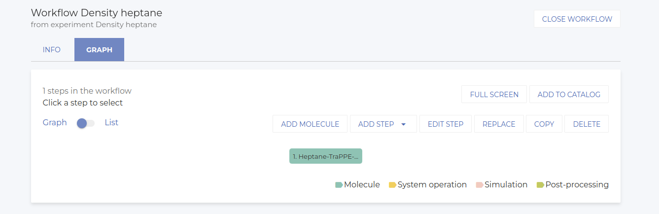
Heptane is already available in the molecule catalog, so click ADD MOLECULE and search for "Heptane-TraPPE-UA" using the filter.
-
Once selected, choose the available potential. In this case we only have one potential available. Please note that we’re using a united atom model to speed up calculations. The workflow at this point is shown below.
-
-
Create and Fill the Simulation Cell:
-
Go to Add Step > Add System Operation and select the Create and fill cell function. This will create the simulation cell and fill it with the heptane molecule.
-
Select the Heptane molecule node as the parent node and proceed without selecting a child step. Click on NEXT.
-
When asked for the children steps, click on NEXT without selecting anything, since we don’t have any children steps in this case.
-
Add a description, if you consider it necessary. Click NEXT.
-
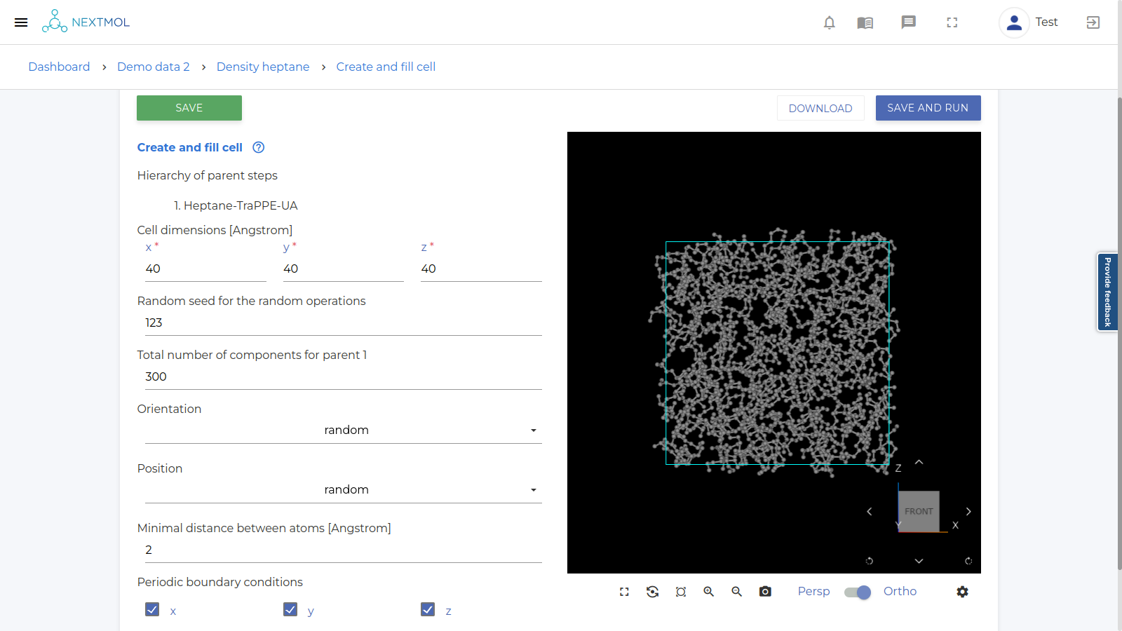
Create a cubic cell with dimensions of 4 nm (i.e. 40 Angstroms in x, y and z directions) and fill it randomly with 300 molecules (Total number of components for parent 1 = 300, orientation = random, position = random). Leave the other parameters as default.
-
Save the setup by clicking SAVE.
-
-
Visualize the System (Optional):
-
Select the node and click EDIT STEP to open the parameters screen.
-
Click SAVE AND RUN to calculate the node[1] and create the cell. Once completed, the visualization will appear (see image below).
-
This visualization step is not necessary for the final scope of the calculation, but it is always good to check that the system has been generated as expected before running the actual simulation.
-
-
Close the node:
-
Once satisfied with the setup, click on
 to close the node and go back to the workflow construction.
-
Next, we will configure the simulation steps. This involves two steps: an energy minimization to relax any unfavorably placed atoms and the production NPT run.
-
Energy Minimization:
-
Go to ADD STEP > Add simulation and select Gromacs simulation.
-
Choose the node with the system (Create and fill cell) as the parent and click NEXT.
-
Leave the children step without selection, and click NEXT.
-
Add a description, if you consider it necessary. Click NEXT.
-
In Run parameters > Calculation mode, select Energy Minimization, which will perform an energy minimization using the steepest descent algorithm. Leave the other parameters as default.
-
Save the configuration by clicking SAVE and close the node.
-
-
NPT Simulation:
-
Again, go to ADD STEP > Add simulation and select Gromacs simulation.
-
Select the previous simulation node (Energy Minimization) as the parent. Leave the children unselected, as in the previous cases.
-
Add a description, if you consider it necessary.
-
Modify the following parameters and leave the rest with their default values:
-
Run parameters:
-
Calculation mode: Choose Molecular Dynamics instead of Energy Minimization.
-
Number of steps: 1,000,000
-
Time step: 2 fs (resulting in a simulation time of 2,000 ps)
-
-
Output control: These values determine how often the code writes to the output files. The following numbers give reasonable results:
-
Frequency for trajectory writing: 5,000
-
Frequency for energy writing: 500
-
Frequency for log writing: 500
-
-
Electrostatics: Since the platform uses GPUs instances, please set VdW calculation mode to Cut-off.
-
Thermostat: Use the v_rescale thermostat at 300 K and generate initial velocities at 300 K.
-
Barostat: Set isotropic C-rescale coupling with a reference pressure of 2 bar and a time constant of 4 ps.
-
-
Save the setup by clicking SAVE.
-
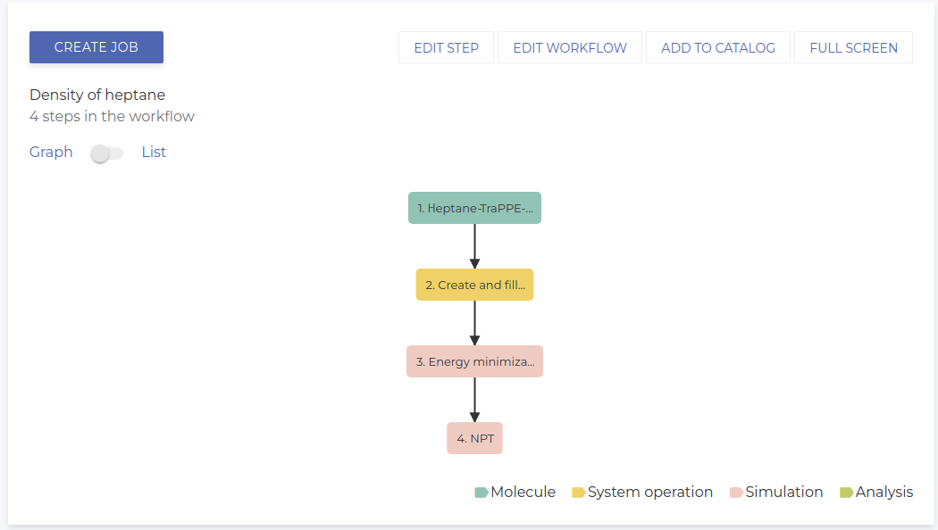
The final workflow is shown below.
Running the simulation and analysis of the results
Now that the setup is complete, we can execute the workflow by creating a job. In the platform, we call JOBs the immutable copies of a workflow that can be executed.
-
Close the workflow by clicking CLOSE WORKFLOW.
-
Select the last node of the workflow and click CREATE JOB to launch the calculation on the cluster.
-
Insert a name for the job, leave the other values on default and save it.
-
Go to the Execution tab and click EXECUTE JOB. The job will complete in a few minutes, and the nodes' statuses will change from "Not submitted" to "Completed". For more information about other states, please read the User Guide.
Once the job is finished, and all the nodes are completed, we can analyze the results:
-
Go to the Graph tab, select the last node, and click NEW ANALYSIS > 2D.
-
Select Time for the X-axis and Density for the Y-axis. Name the analysis and save it.
-
After running the analysis, go to the Visualize tab to view the 2D plot of the results (see image below).
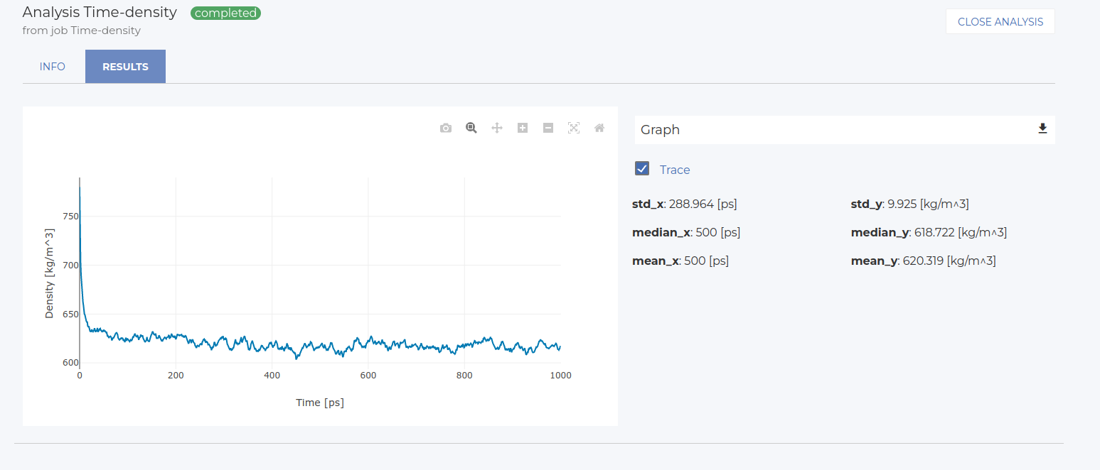
Statistics on this plot are reported on the right side of the screen. In this case, for instance, the mean density value is approximately 619 kg/m3, with a standard deviation of about 10 kg/m3. These values may vary slightly between runs.